Kinematics Notes | Physics HL

Describing motion with quantities and graphs

Kinematics describes how an object moves without first explaining the forces that cause the motion. Every description needs a reference frame: choose an origin, label a positive direction, and measure time from a stated instant. Once that choice is made, position, displacement, velocity and acceleration can carry positive or negative signs.

A motion description should connect four representations: words, a diagram, equations and graphs. For example, “the cyclist is moving west and slowing down” means velocity points west while acceleration points east. A correct answer is more than a number: its sign, direction and unit are part of the physics.

On a position–time graph the gradient gives velocity. On a velocity–time graph the gradient gives acceleration and the signed area gives displacement. On an acceleration–time graph the signed area gives the change in velocity. These links let you move between a story of the motion and measurable quantities.

Key terms

Kinematics: The description of motion using quantities such as position, velocity and acceleration.
Reference frame: The chosen origin, axes and clock relative to which motion is measured.
Position: An object's location relative to the chosen origin.
Gradient: The rate at which the vertical graph quantity changes with the horizontal graph quantity.

Worked examples

Reading a velocity–time graph

A cyclist accelerates uniformly from $2.0\,\mathrm{m\,s^{-1}}$ to $10.0\,\mathrm{m\,s^{-1}}$ in $4.0\,\mathrm{s}$ . Find the acceleration and displacement.

1Acceleration is the gradient: $a=\frac{(10.0-2.0)}{4.0}=2.0\,\mathrm{m\,s^{-2}}$ .
2Displacement is the trapezium area under the velocity–time graph: $s=\tfrac12(2.0+10.0)(4.0)=24\,\mathrm{m}$ .
3Both velocities are positive, so all of this signed area also contributes to distance travelled.

Answer: The acceleration is $2.0\,\mathrm{m\,s^{-2}}$ and the displacement is $24\,\mathrm{m}$ in the positive direction.

Rules and formulas

Displacement from position

\Delta x=x_{\mathrm{f}}-x_{\mathrm{i}}

$\Delta x$: displacement ( $m$ )
$x_{\mathrm{f}}$: final position ( $m$ )
$x_{\mathrm{i}}$: initial position ( $m$ )

Average acceleration

\bar{a}=\frac{\Delta v}{\Delta t}

$\bar{a}$: average acceleration ( $m s⁻²$ )
$\Delta v$: change in velocity ( $m s⁻¹$ )
$\Delta t$: elapsed time ( $s$ )

Reference frames, distance and displacement

Distance is the total length of the path travelled. It is a scalar, so it is non-negative and has no direction. Displacement is the change from initial to final position. It is a vector and depends only on the endpoints, not on the route taken.

In one dimension a sign communicates direction: if east is positive, $+20\,\mathrm{m}$ means $20\,\mathrm{m}$ east and $-20\,\mathrm{m}$ means $20\,\mathrm{m}$ west. In two dimensions displacement is drawn as a straight arrow from the initial point to the final point, even when the actual path is curved.

Speed is the rate at which distance is covered, whereas velocity is the rate of change of displacement. Speed can be zero or positive but never negative. Velocity can be positive, negative or zero because it includes direction.

Key terms

Scalar: A physical quantity described completely by magnitude and unit.
Vector: A physical quantity with magnitude, direction and unit.
Distance: The total scalar path length travelled.
Displacement: The vector change from initial to final position.
Speed: The rate at which distance is travelled.
Velocity: The rate of change of displacement.

Worked examples

Walking out and partly back

A student walks $30\,\mathrm{m}$ east and then $10\,\mathrm{m}$ west in $20\,\mathrm{s}$ . Take east as positive. Find distance, displacement, average speed and average velocity.

1Distance adds path lengths: $30+10=40\,\mathrm{m}$ .
2Displacement adds signed changes: $+30-10=+20\,\mathrm{m}$ , or $20\,\mathrm{m}$ east.
3Average speed is $\frac{40}{20}=2.0\,\mathrm{m\,s^{-1}}$ .
4Average velocity is $\frac{+20}{20}=+1.0\,\mathrm{m\,s^{-1}}$ , or $1.0\,\mathrm{m\,s^{-1}}$ east.

Answer: Distance $=40\,\mathrm{m}$ ; displacement $=20\,\mathrm{m}$ east; average speed $=2.0\,\mathrm{m\,s^{-1}}$ ; average velocity $=1.0\,\mathrm{m\,s^{-1}}$ east.

One complete lap

A runner completes one $400\,\mathrm{m}$ track lap in $80\,\mathrm{s}$ and finishes at the starting line. Compare average speed and average velocity.

1The distance is one lap: $400\,\mathrm{m}$ .
2Initial and final positions are the same, so displacement is zero.
3Average speed is $\frac{400}{80}=5.0\,\mathrm{m\,s^{-1}}$ , but average velocity is $\frac{0}{80}=0$ .

Answer: Average speed is $5.0\,\mathrm{m\,s^{-1}}$ ; average velocity is zero.

Rules and formulas

Average speed

\text{average speed}=\frac{\text{total distance}}{\Delta t}

$\Delta t$: total elapsed time ( $s$ )

Average velocity

\bar{v}=\frac{\Delta x}{\Delta t}

$\bar{v}$: average velocity ( $m s⁻¹$ )
$\Delta x$: displacement ( $m$ )
$\Delta t$: elapsed time ( $s$ )

Average and instantaneous speed, velocity and acceleration

An average value describes a whole time interval. An instantaneous value describes one moment. A journey computer may report an average speed of $60\,\mathrm{km\,h^{-1}}$ , while the speedometer gives the instantaneous speed right now.

On a position–time graph, average velocity is the gradient of a secant line joining two points. Instantaneous velocity is the gradient of the tangent at one point—the value approached as the time interval becomes very small. The same idea links a velocity–time graph to instantaneous acceleration.

Acceleration measures a change in velocity, so it can result from a change in speed, direction, or both. In one-dimensional motion, compare the signs of velocity and acceleration: the object speeds up when the signs match and slows down when the signs are opposite.

Key terms

Average quantity: A change or total divided by the duration of a finite interval.
Instantaneous quantity: The value at a particular moment, represented by a tangent gradient on the relevant graph.
Acceleration: The rate of change of velocity; a vector measured in metres per second squared.
Uniform acceleration: Acceleration that remains constant with time.
Non-uniform acceleration: Acceleration that changes in magnitude or direction with time.

Worked examples

Stopping and reversing

A trolley's velocity changes from $+14\,\mathrm{m\,s^{-1}}$ to $-6.0\,\mathrm{m\,s^{-1}}$ in $5.0\,\mathrm{s}$ . Find its average acceleration and interpret the signs.

1The velocity change is $\Delta v=-6.0-(+14)=-20\,\mathrm{m\,s^{-1}}$ .
2Average acceleration is $\bar a=\frac{-20}{5.0}=-4.0\,\mathrm{m\,s^{-2}}$ .
3The final negative velocity shows that the trolley passed through rest and then moved in the negative direction; it did not merely slow to $6.0\,\mathrm{m\,s^{-1}}$ .

Answer: The average acceleration is $-4.0\,\mathrm{m\,s^{-2}}$ , opposite the chosen positive direction.

Instantaneous values from a model

A particle's position is $x=2t^2+1$ , with $x$ in metres and $t$ in seconds. Find its velocity and acceleration at $t=3.0\,\mathrm{s}$ .

1The instantaneous velocity is the position–time tangent gradient: $v=\frac{\mathrm{d}x}{\mathrm{d}t}=4t$ .
2At $t=3.0\,\mathrm{s}$ , $v=12\,\mathrm{m\,s^{-1}}$ .
3Acceleration is the velocity–time gradient: $a=\frac{\mathrm{d}v}{\mathrm{d}t}=4.0\,\mathrm{m\,s^{-2}}$ .

Answer: At $3.0\,\mathrm{s}$ , velocity is $12\,\mathrm{m\,s^{-1}}$ and acceleration is $4.0\,\mathrm{m\,s^{-2}}$ .

Rules and formulas

Instantaneous velocity

v=\frac{\mathrm{d}x}{\mathrm{d}t}

$v$: instantaneous velocity ( $m s⁻¹$ )
$x$: position ( $m$ )
$t$: time ( $s$ )

Instantaneous acceleration

a=\frac{\mathrm{d}v}{\mathrm{d}t}

$a$: instantaneous acceleration ( $m s⁻²$ )
$v$: velocity ( $m s⁻¹$ )

Speed from one-dimensional velocity

\text{speed}=|v|

$v$: signed velocity ( $m s⁻¹$ )

Position–time, velocity–time and acceleration–time graphs

A position–time graph shows where an object is. A horizontal segment means constant position and therefore zero velocity. A straight sloping segment means constant velocity. A curve whose gradient becomes steeper shows increasing speed; whether velocity is positive or negative depends on the slope's sign.

A velocity–time graph shows both speed and direction. Its gradient gives acceleration. The signed area between the graph and time axis gives displacement: area above the axis is positive and area below it is negative. Total distance is found by adding the magnitudes of all areas, so negative parts are counted positively.

An acceleration–time graph shows how velocity changes. Its signed area over an interval is $\Delta v$ . A zero acceleration line means constant velocity, not necessarily zero velocity. A position–time graph can decrease, but a cumulative distance–time graph cannot.

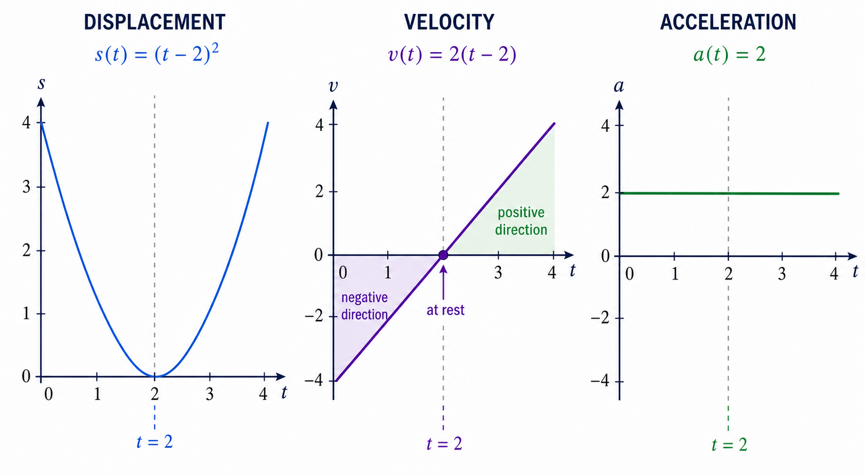Three aligned motion graphs for displacement s equals t minus two squared, velocity v equals two times t minus two, and constant acceleration two, showing reversal at t equals two. Read vertically at the same time: the gradient of the displacement graph is velocity, and the gradient of the velocity graph is acceleration. At $t=2$ the particle is instantaneously at rest and reverses direction.

Open graph full size

Key terms

Tangent: A line touching a curve locally whose gradient gives an instantaneous rate of change.
Signed area: Area above the time axis counted positive and area below counted negative.
Turning point: A position where velocity becomes zero and changes sign, so the direction of motion reverses.

Worked examples

Signed area and total distance

A velocity–time graph shows $+6.0\,\mathrm{m\,s^{-1}}$ from $0$ to $4.0\,\mathrm{s}$ , a uniform change from $+6.0$ to $-6.0\,\mathrm{m\,s^{-1}}$ from $4.0$ to $6.0\,\mathrm{s}$ , then $-6.0\,\mathrm{m\,s^{-1}}$ from $6.0$ to $8.0\,\mathrm{s}$ . Find displacement, distance and the middle-interval acceleration.

1First interval area: $(+6.0)(4.0)=+24\,\mathrm{m}$ .
2During the middle interval the equal positive and negative triangular areas cancel, so its net displacement is zero but its distance is $3.0+3.0=6.0\,\mathrm{m}$ .
3Final interval area: $(-6.0)(2.0)=-12\,\mathrm{m}$ .
4Displacement is $+24+0-12=+12\,\mathrm{m}$ ; distance is $24+6+12=42\,\mathrm{m}$ .
5The middle gradient is $a=\frac{(-6.0-6.0)}{(6.0-4.0)}=-6.0\,\mathrm{m\,s^{-2}}$ .

Answer: Displacement $=+12\,\mathrm{m}$ , distance $=42\,\mathrm{m}$ , and middle-interval acceleration $=-6.0\,\mathrm{m\,s^{-2}}$ .

A graph that returns to its starting position

For $0\le t\le4$ , a particle has position $x=(t-2)^2$ metres. Find net displacement and total distance over the interval.

1At $t=0$ , $x=4\,\mathrm{m}$ ; at $t=2$ , $x=0$ ; at $t=4$ , $x=4\,\mathrm{m}$ .
2Net displacement is final minus initial position: $4-4=0$ .
3The particle travels $4\,\mathrm{m}$ toward the origin and $4\,\mathrm{m}$ back, so distance is $8\,\mathrm{m}$ .
4Because $v=2(t-2)$ , velocity changes from negative to positive at $t=2$ , confirming the reversal.

Answer: Net displacement is zero; total distance is $8\,\mathrm{m}$ .

Rules and formulas

Velocity from a position–time graph

v=\text{gradient of the }x\text{-}t\text{ graph}

$v$: instantaneous velocity ( $m s⁻¹$ )

Displacement from a velocity–time graph

\Delta x=\int_{t_1}^{t_2}v\,\mathrm{d}t

$\Delta x$: signed area under the velocity–time graph ( $m$ )

Distance from a velocity–time graph

\text{distance}=\int_{t_1}^{t_2}|v|\,\mathrm{d}t

$|v|$: speed ( $m s⁻¹$ )

Velocity change from an acceleration–time graph

\Delta v=\int_{t_1}^{t_2}a\,\mathrm{d}t

$\Delta v$: signed area under the acceleration–time graph ( $m s⁻¹$ )

Constant-acceleration equations (SUVAT)

For motion with constant acceleration, five signed quantities describe one straight-line component: initial velocity $u$ , final velocity $v$ , acceleration $a$ , displacement $s$ and elapsed time $t$ . The four SUVAT equations are different combinations of the same velocity–time graph.

Choose an equation by listing known values and the required unknown. Use the equation that omits the quantity you neither know nor need. For example, if time is absent from the data and answer, $v^2=u^2+2as$ is often the direct route.

The model is valid only while acceleration is constant. It works for free fall when air resistance is negligible and for each independent component of ideal projectile motion. It does not describe a full interval in which drag changes, an engine produces changing acceleration, or the acceleration direction varies.

A reliable workflow is: draw the positive axis; sketch the motion; list $u,v,a,s,t$ with signs and SI units; select the equation; solve algebraically; then interpret signs and reject any unphysical root.

Key terms

Initial velocity, $u$: Velocity at the start of the chosen constant-acceleration interval.
Final velocity, $v$: Velocity at the end of the chosen interval.
Displacement, $s$: Signed change in position during the interval.
Constant acceleration model: A model in which the velocity changes by equal amounts in equal time intervals.

Worked examples

Accelerating bicycle

A bicycle has initial velocity $3.0\,\mathrm{m\,s^{-1}}$ and accelerates at $1.5\,\mathrm{m\,s^{-2}}$ for $6.0\,\mathrm{s}$ . Find final velocity and displacement.

1Use $v=u+at$ : $v=3.0+(1.5)(6.0)=12\,\mathrm{m\,s^{-1}}$ .
2Use $s=ut+\tfrac12at^2$ : $s=(3.0)(6.0)+\tfrac12(1.5)(6.0)^2$ .
3This gives $s=18+27=45\,\mathrm{m}$ .

Answer: Final velocity $=12\,\mathrm{m\,s^{-1}}$ ; displacement $=45\,\mathrm{m}$ .

Emergency braking

A car travelling at $22\,\mathrm{m\,s^{-1}}$ brakes with constant acceleration $-5.5\,\mathrm{m\,s^{-2}}$ . Find stopping time and braking displacement.

1Take forward as positive: $u=+22$ , $v=0$ , $a=-5.5\,\mathrm{m\,s^{-2}}$ .
2From $v=u+at$ , $t=\frac{(0-22)}{(-5.5)}=4.0\,\mathrm{s}$ .
3From $v^2=u^2+2as$ , $s=\frac{(0-22^2)}{(2\times-5.5)}=44\,\mathrm{m}$ .
4Check: constant acceleration makes average velocity $\frac{(u+v)}{2}=11\,\mathrm{m\,s^{-1}}$ , and $(11)(4.0)=44\,\mathrm{m}$ .

Answer: Stopping time $=4.0\,\mathrm{s}$ ; braking displacement $=44\,\mathrm{m}$ forward.

Rules and formulas

Displacement from mean velocity

s=\frac{1}{2}(u+v)t

$s$: displacement ( $m$ )
$u$: initial velocity ( $m s⁻¹$ )
$v$: final velocity ( $m s⁻¹$ )
$t$: elapsed time ( $s$ )

Velocity after time

v=u+at

$a$: constant acceleration ( $m s⁻²$ )

Displacement after time

s=ut+\frac{1}{2}at^2

$s$: displacement ( $m$ )
$u$: initial velocity ( $m s⁻¹$ )
$a$: constant acceleration ( $m s⁻²$ )
$t$: elapsed time ( $s$ )

Time-independent equation

v^2=u^2+2as

$v$: final velocity ( $m s⁻¹$ )
$u$: initial velocity ( $m s⁻¹$ )
$a$: constant acceleration ( $m s⁻²$ )
$s$: displacement ( $m$ )

Free fall and vertical motion near Earth

Free fall means gravity is the only significant influence on the motion. Near Earth's surface and over modest height changes, the acceleration has approximately constant magnitude $g=9.81\,\mathrm{m\,s^{-2}}$ and points downward. When air resistance is negligible, all objects have the same free-fall acceleration regardless of mass.

The sign of gravitational acceleration comes from your axis. If upward is positive, $a_y=-g$ ; if downward is positive, $a_y=+g$ . The symbol $g$ usually means the positive magnitude, so do not automatically type $-9.81$ without first choosing the axis.

For an object thrown upward, the upward velocity decreases to zero at the highest point and then becomes downward. At the top, velocity is zero for one instant but acceleration is still downward with magnitude $g$ . If it returns to the same height without drag, its speed there equals its launch speed and the upward and downward times are equal.

Key terms

Free fall: Motion in which gravity is the only significant influence.
Gravitational field strength, $g$: Gravitational force per unit mass, measured in $\mathrm{N\,kg^{-1}}$ . Its numerical value equals free-fall acceleration in $\mathrm{m\,s^{-2}}$ ; near Earth its magnitude is about $9.81$ .
Highest point: The instant at which the vertical velocity is zero before reversing direction.

Worked examples

Dropped from a height

A ball is released from rest $45\,\mathrm{m}$ above the ground. Ignore air resistance. Find fall time and impact speed.

1Choose downward as positive: $u=0$ , $a=+9.81\,\mathrm{m\,s^{-2}}$ , $s=+45\,\mathrm{m}$ .
2From $s=ut+\tfrac12at^2$ , $45=\tfrac12(9.81)t^2$ , so $t=3.03\,\mathrm{s}$ .
3Then $v=u+at=(9.81)(3.03)=29.7\,\mathrm{m\,s^{-1}}$ downward.

Answer: Fall time $=3.03\,\mathrm{s}$ ; impact speed $=29.7\,\mathrm{m\,s^{-1}}$ .

Thrown straight upward

A ball is launched vertically upward at $14.0\,\mathrm{m\,s^{-1}}$ . Ignore drag. Find time to the highest point, maximum rise and return time to the launch height.

1Take upward as positive: $u=+14.0\,\mathrm{m\,s^{-1}}$ , $v=0$ at the top and $a=-9.81\,\mathrm{m\,s^{-2}}$ .
2From $v=u+at$ , $t_{\text{top}}=\frac{14.0}{9.81}=1.43\,\mathrm{s}$ .
3From $v^2=u^2+2as$ , $0=14.0^2+2(-9.81)s$ , so $s=9.99\,\mathrm{m}$ .
4The no-drag motion is time-symmetric at the launch height. Retain the unrounded time: $T=2\left(\frac{14.0}{9.81}\right)\approx2.85\,\mathrm{s}$ , rather than doubling the displayed rounded value.

Answer: Time to top $=1.43\,\mathrm{s}$ ; maximum rise $=9.99\,\mathrm{m}$ ; return time $=2.85\,\mathrm{s}$ .

Rules and formulas

Vertical acceleration with upward positive

a_y=-g\approx-9.81\,\mathrm{m\,s^{-2}}

$a_y$: vertical acceleration ( $m s⁻²$ )
$g$: magnitude of free-fall acceleration ( $m s⁻²$ )

Projectile motion in two dimensions

An ideal projectile is an object that, after launch, moves under gravity alone; air resistance is neglected in this model. Measure the launch angle $\theta$ from the positive horizontal and resolve the initial velocity: $u_x=u\cos\theta$ , $u_y=u\sin\theta$ . The two components share the same time but follow different motion rules.

Horizontally, $a_x=0$ , so $v_x=u_x$ is constant. Vertically, $a_y=-g$ if upward is positive, so $v_y=u_y-gt$ . Combining the simultaneous horizontal and vertical positions produces a parabolic path when drag is absent, though the trajectory equation does not need to be derived.

The velocity vector is always tangent to the path. At the apex of an angled projectile, $v_y=0$ , but $v_x$ remains non-zero, so the projectile is still moving and its acceleration is still downward. For a launch below the horizontal, enter the vertical component as negative when upward is positive.

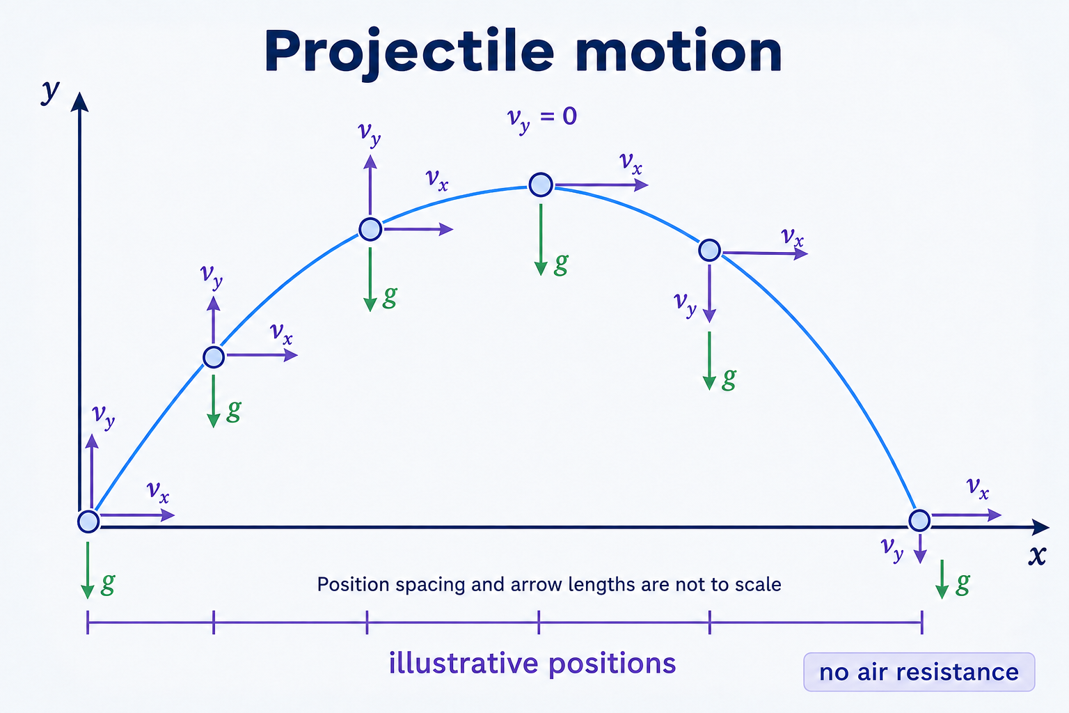Qualitative projectile sketch: horizontal velocity points right, vertical velocity points upward on ascent, is zero at the apex, and points downward on descent; gravity always points downward. Position spacing and arrow lengths are not to scale. This is a qualitative sketch, not an equal-time position plot; do not measure speed or acceleration from its spacing or arrow lengths. In the ideal uniform-gravity, no-drag model, equal time intervals give equal horizontal displacements because $v_x$ is constant. The vertical component changes by $\Delta v_y=-g\Delta t$ : upward on ascent, zero at the apex, then increasingly downward. Acceleration remains downward with constant magnitude $g$ .

Open graph full size

Key terms

Projectile: An object moving under gravity after launch, with other effects neglected in the ideal model.
Component: The part of a vector along a chosen axis.
Trajectory: The path followed by a moving object.
Apex: The highest point of a projectile trajectory, where the vertical velocity component is momentarily zero.

Worked examples

Angled launch returning to the same height

A ball is launched at $20.0\,\mathrm{m\,s^{-1}}$ , $35.0^\circ$ above the horizontal, and lands at the launch height. Ignore drag. Find time of flight, range and maximum height.

1Resolve the launch velocity: $u_x=20.0\cos35.0^\circ=16.4\,\mathrm{m\,s^{-1}}$ and $u_y=20.0\sin35.0^\circ=11.5\,\mathrm{m\,s^{-1}}$ .
2At the top, $v_y=0$ , so $t_{\text{top}}=\frac{u_y}{g}=1.17\,\mathrm{s}$ . Returning to the same height takes $T=2t_{\text{top}}=2.34\,\mathrm{s}$ .
3Use unrounded components and flight time: $R=\frac{(20.0)^2\sin(70.0^\circ)}{9.81}\approx38.3\,\mathrm{m}$ . The displayed rounded values $16.4$ and $2.34$ are not the values carried into this calculation.
4Maximum height above launch is $H=\frac{u_y^2}{(2g)}=6.71\,\mathrm{m}$ .

Answer: Time of flight $=2.34\,\mathrm{s}$ , range $=38.3\,\mathrm{m}$ , maximum height $=6.71\,\mathrm{m}$ .

Horizontal launch from a cliff

A package leaves a $20.0\,\mathrm{m}$ -high platform horizontally at $8.0\,\mathrm{m\,s^{-1}}$ . Ignore drag. Find fall time, horizontal range and impact speed.

1Vertical motion sets the time: $20.0=\tfrac12gt^2$ , giving $t=2.02\,\mathrm{s}$ .
2Horizontal velocity is constant, so $x=(8.0)(2.02)=16.2\,\mathrm{m}$ .
3The vertical impact velocity is $v_y=-gt=-19.8\,\mathrm{m\,s^{-1}}$ ; the horizontal component remains $+8.0\,\mathrm{m\,s^{-1}}$ .
4Impact speed is $\sqrt{v_x^2+v_y^2}=\sqrt{8.0^2+19.8^2}=21.4\,\mathrm{m\,s^{-1}}$ .

Answer: Fall time $=2.02\,\mathrm{s}$ , range $=16.2\,\mathrm{m}$ , impact speed $=21.4\,\mathrm{m\,s^{-1}}$ .

Launch below the horizontal

A ball is thrown to the right at $15.0\,\mathrm{m\,s^{-1}}$ , $20.0^\circ$ below the horizontal. With right and up positive, write its initial components.

1The horizontal component points right: $u_x=15.0\cos20.0^\circ=+14.1\,\mathrm{m\,s^{-1}}$ .
2The vertical component points down: $u_y=-15.0\sin20.0^\circ=-5.13\,\mathrm{m\,s^{-1}}$ .
3Gravity is also downward, so $a_y=-9.81\,\mathrm{m\,s^{-2}}$ .

Answer: $u_x=+14.1\,\mathrm{m\,s^{-1}}$ , $u_y=-5.13\,\mathrm{m\,s^{-1}}$ .

Rules and formulas

Initial velocity components

u_x=u\cos\theta,\qquad u_y=u\sin\theta

$u$: initial speed ( $m s⁻¹$ )
$\theta$: launch angle measured from the positive horizontal ( $°$ )

Ideal horizontal motion

x=x_0+u_xt,\qquad v_x=u_x

$x_0$: initial horizontal position ( $m$ )
$u_x$: horizontal velocity component ( $m s⁻¹$ )

Ideal vertical motion

y=y_0+u_yt-\frac{1}{2}gt^2,\qquad v_y=u_y-gt

$y_0$: initial vertical position ( $m$ )
$u_y$: initial vertical velocity component ( $m s⁻¹$ )
$g$: free-fall acceleration magnitude ( $m s⁻²$ )

Speed from perpendicular components

v=\sqrt{v_x^2+v_y^2}

$v$: speed ( $m s⁻¹$ )
$v_x$: horizontal velocity component ( $m s⁻¹$ )
$v_y$: vertical velocity component ( $m s⁻¹$ )

Flight time, range and maximum rise: check the conditions

T=\frac{2u\sin\theta}{g},\quad R=\frac{u^2\sin(2\theta)}{g},\quad H=\frac{u^2\sin^2\theta}{2g}

$T$: time of flight ( $s$ )
$R$: horizontal range ( $m$ )
$H$: maximum height above launch ( $m$ )

Fluid resistance and terminal speed

A fluid is a liquid or a gas. Fluid resistance, often called drag, acts opposite an object's velocity relative to the fluid. Its magnitude generally increases with speed and also depends on shape, frontal area and the fluid. Therefore drag usually makes acceleration non-uniform.

For the usual upward-launched projectile in still air, drag opposes the velocity relative to the air. Horizontal speed decreases, maximum rise and range are reduced, and the trajectory is no longer the ideal symmetric parabola. A moving fluid, such as a tailwind, changes this comparison. Drag also changes time of flight: do not assume the same-height no-drag formula or that ascent and descent take equal times. For a horizontal launch from a given height in still air, upward drag during the fall delays impact compared with the no-drag model. Other launch conditions need their own comparison; a shorter range alone does not prove a shorter flight time. Quantitative SUVAT projectile calculations require negligible drag.

For an object falling vertically from rest, weight initially exceeds the upward drag, so it accelerates downward. As speed grows, drag grows and the resultant force and acceleration shrink. At terminal speed, the upward fluid forces balance weight, the resultant force is zero and acceleration is zero—but the object continues downward at a constant non-zero speed.

In still air, an object moving vertically upward has both weight and drag downward and slows faster than in ideal free fall. For a vertical throw in still air, drag is momentarily zero at the highest point because the relative velocity is zero. With wind, being at rest relative to the ground does not guarantee zero drag. An angled projectile retains horizontal speed at its apex, so drag can still act there.

Key terms

Fluid resistance (drag): A force opposing motion relative to a gas or liquid.
Terminal speed: The constant non-zero speed reached when the resultant force and acceleration are zero.
Resultant force: The vector sum of all forces acting on an object.
Non-uniform acceleration: Acceleration that changes as the forces or direction of motion change.

Worked examples

Reading a skydiver's velocity–time graph

In still air, a skydiver starts from rest, speeds up, then approaches a constant downward velocity. Neglect buoyancy. Explain how the graph gradient and drag change.

1At release, speed and drag are near zero, so downward acceleration is close to $g$ and the velocity–time graph is steep.
2As downward speed increases, upward drag increases. The resultant force shrinks, so the graph's gradient becomes less steep.
3At terminal speed, velocity is constant and the graph is horizontal. Its gradient—and therefore acceleration—is zero.

Answer: The graph approaches a horizontal line because increasing drag reduces acceleration to zero at a non-zero terminal velocity.

Opening a parachute

A skydiver is descending at terminal speed in still air when a parachute opens. Neglect buoyancy. Describe the acceleration immediately after deployment and the later motion.

1The parachute greatly increases area, so upward drag suddenly exceeds weight.
2The resultant force and acceleration point upward while velocity is still downward, so the skydiver's speed decreases.
3As the speed decreases, drag decreases until it balances weight again at a new, much lower terminal speed.

Answer: The skydiver first decelerates strongly, then settles to a lower constant downward terminal speed.

Rules and formulas

Terminal-speed condition

F_{\mathrm{resultant}}=0\quad\Rightarrow\quad a=0

$F_{\mathrm{resultant}}$: vector sum of forces ( $N$ )
$a$: acceleration ( $m s⁻²$ )

Simplified vertical balance

F_{\mathrm{drag}}=mg\quad\text{at terminal speed (if buoyancy is negligible)}

$F_{\mathrm{drag}}$: drag magnitude ( $N$ )
$m$: mass ( $kg$ )
$g$: gravitational field strength ( $N kg⁻¹$ )

Practical kinematics, data and model limits

Video analysis and motion sensors turn position measurements into motion graphs. Calibrate a length scale, choose axes, record position at known times, plot $x$ against $t$ , then obtain velocity from gradients. Plotting velocity against time reveals whether acceleration is approximately constant: a straight best-fit line supports that model.

Measurements have uncertainty. Sources include limited pixel or sensor resolution, frame timing, perspective/parallax and poor scale calibration. An inconsistent release can introduce trial-to-trial variation. Air resistance is a limitation of a no-drag model, not an instrument uncertainty. Use widely separated points on a best-fit line to reduce the fractional uncertainty in its gradient.

A model is useful because it deliberately ignores small effects, but its assumptions must be stated. Constant $g$ , a point-like object, a flat local surface and negligible drag can be excellent for a short classroom projectile; they may fail for a feather, a long fall or high-speed motion.

Key terms

Model: A simplified description that keeps the effects important for a particular situation.
Uncertainty: A quantified range representing the limits of a measurement.
Best-fit line: A line representing the overall trend of data rather than joining every point.
Parallax: An apparent position shift caused by viewing a scale or object from an angle.

Worked examples

Average velocity with measurement uncertainty

A cart is at $x_1=(0.20\pm0.01)\,\mathrm{m}$ when $t_1=(0.50\pm0.01)\,\mathrm{s}$ , and at $x_2=(1.40\pm0.01)\,\mathrm{m}$ when $t_2=(2.00\pm0.01)\,\mathrm{s}$ . Estimate average velocity and its worst-case uncertainty.

1 $\Delta x=1.40-0.20=1.20\,\mathrm{m}$ , with absolute uncertainty $0.01+0.01=0.02\,\mathrm{m}$ .
2 $\Delta t=2.00-0.50=1.50\,\mathrm{s}$ , also with uncertainty $0.02\,\mathrm{s}$ .
3Average velocity is $\frac{1.20}{1.50}=0.80\,\mathrm{m\,s^{-1}}$ .
4For the first-order worst-case estimate for a quotient, add fractional uncertainties: $\frac{0.02}{1.20}+\frac{0.02}{1.50}=0.030$ . Hence $\delta\bar v\approx(0.030)(0.80)=0.024\,\mathrm{m\,s^{-1}}$ , reported as $0.02\,\mathrm{m\,s^{-1}}$ to one significant figure. This is an approximate propagation rule, not an exact bound.

Answer: $\bar v\approx(0.80\pm0.02)\,\mathrm{m\,s^{-1}}$ .

Thinking distance plus braking distance

A car moves at $18\,\mathrm{m\,s^{-1}}$ . The driver's reaction time is $0.75\,\mathrm{s}$ , after which the car brakes uniformly at $-4.5\,\mathrm{m\,s^{-2}}$ . Find total stopping distance.

1During reaction time, velocity is constant: $s_{\text{reaction}}=(18)(0.75)=13.5\,\mathrm{m}$ .
2During braking, use $v^2=u^2+2as$ : $0=18^2+2(-4.5)s$ , so $s_{\text{braking}}=36.0\,\mathrm{m}$ .
3Add distances from the two different models: $13.5+36.0=49.5\,\mathrm{m}$ .

Answer: The total stopping distance is $49.5\,\mathrm{m}$ .

Exam workflow and mixed applications

Begin by identifying the physical model: constant velocity, constant acceleration, ideal projectile motion, or motion with drag. Write the assumptions that make the model valid. Then draw a labelled sketch, choose axes and convert all data to compatible SI units.

Keep vector signs through the algebra. A negative displacement, velocity or acceleration can be the correct physical result. At the end, give a direction in words where helpful, round to sensible significant figures, and check that the magnitude and unit are realistic.

Use more than one representation as a check. A SUVAT displacement should agree with the area beneath the corresponding velocity–time graph. A projectile's horizontal and vertical results must refer to the same time. A terminal-speed description must have zero acceleration but non-zero velocity.

Key terms

Sign convention: A declared choice of positive directions used consistently throughout a solution.
Physical root: A mathematical solution that is valid for the stated time interval and situation.
Dimensional check: A check that an equation or answer has the required physical units.

Worked examples

Three-stage train journey

A train starts from rest, accelerates at $2.0\,\mathrm{m\,s^{-2}}$ for $5.0\,\mathrm{s}$ , travels at constant speed for $12\,\mathrm{s}$ , then brakes at $-2.5\,\mathrm{m\,s^{-2}}$ to rest. Find total distance and average speed.

1Stage 1: $v=(2.0)(5.0)=10\,\mathrm{m\,s^{-1}}$ and $s_1=\tfrac12(2.0)(5.0)^2=25\,\mathrm{m}$ .
2Stage 2: $s_2=vt=(10)(12)=120\,\mathrm{m}$ .
3Stage 3: braking time is $\frac{(0-10)}{(-2.5)}=4.0\,\mathrm{s}$ , and $s_3=\tfrac12(10+0)(4.0)=20\,\mathrm{m}$ .
4Total distance is $25+120+20=165\,\mathrm{m}$ ; total time is $5.0+12+4.0=21\,\mathrm{s}$ .
5Average speed is $\frac{165}{21}=7.86\,\mathrm{m\,s^{-1}}$ .

Answer: Total distance $=165\,\mathrm{m}$ ; average speed $=7.86\,\mathrm{m\,s^{-1}}$ .

Vertical launch from a balcony

A ball is thrown upward at $12.0\,\mathrm{m\,s^{-1}}$ from a balcony $8.0\,\mathrm{m}$ above the ground. Ignore drag. Find the time to reach the ground and the impact velocity.

1Choose upward positive and ground at $y=0$ : $y=8.0+12.0t-4.905t^2$ .
2Set $y=0$ at impact and solve $4.905t^2-12.0t-8.0=0$ . The roots are about $2.99\,\mathrm{s}$ and $-0.55\,\mathrm{s}$ .
3Reject the negative root because it refers to the extrapolated motion before launch.
4Impact velocity is $v_y=u_y-gt=12.0-(9.81)(2.99)=-17.3\,\mathrm{m\,s^{-1}}$ .

Answer: The ball reaches the ground after $2.99\,\mathrm{s}$ with velocity $-17.3\,\mathrm{m\,s^{-1}}$ , meaning $17.3\,\mathrm{m\,s^{-1}}$ downward.

Topic summary

Kinematics describes motion relative to a chosen origin, axes and clock.
Distance is total scalar path length; displacement is the vector change in position.
Average speed uses total distance, while average velocity uses displacement.
Instantaneous velocity is the tangent gradient of a position–time graph; instantaneous acceleration is the tangent gradient of a velocity–time graph.
An object speeds up when velocity and acceleration point in the same direction and slows down when they point in opposite directions.
The signed area under a velocity–time graph is displacement; adding area magnitudes gives distance.
The signed area under an acceleration–time graph is the change in velocity.
The four SUVAT equations apply only when acceleration is constant over the interval or component being analysed.
Near Earth, free-fall acceleration has magnitude $g\approx9.81\,\mathrm{m\,s^{-2}}$ downward; its algebraic sign depends on the chosen axis.
At the top of a vertical throw or projectile, $v_y=0$ but vertical acceleration remains downward.
Ideal projectile motion combines constant horizontal velocity with constant downward vertical acceleration using one shared time.
For launches below the horizontal, the initial vertical component is negative when upward is positive.
Drag acts opposite velocity relative to a fluid, makes acceleration variable and produces a non-parabolic, asymmetric projectile path.
At terminal speed, resultant force and acceleration are zero while velocity remains constant and non-zero.
State model assumptions, use a consistent sign convention, keep SI units and interpret every sign and root physically.