Eigenvalues, eigenvectors and diagonalization

An eigenvector remains on its original line through the origin after multiplication by $A$. Its direction is preserved up to possible reversal.

If $\lambda>1$, the vector stretches; if $0<\lambda<1$, it contracts; if $\lambda<0$, it reverses and scales by $|\lambda|$. If $\lambda=0$, it collapses to the origin.

A general vector need not preserve its direction. When a matrix has a basis of eigenvectors, a general vector can be decomposed along those eigendirections and each component evolves independently.

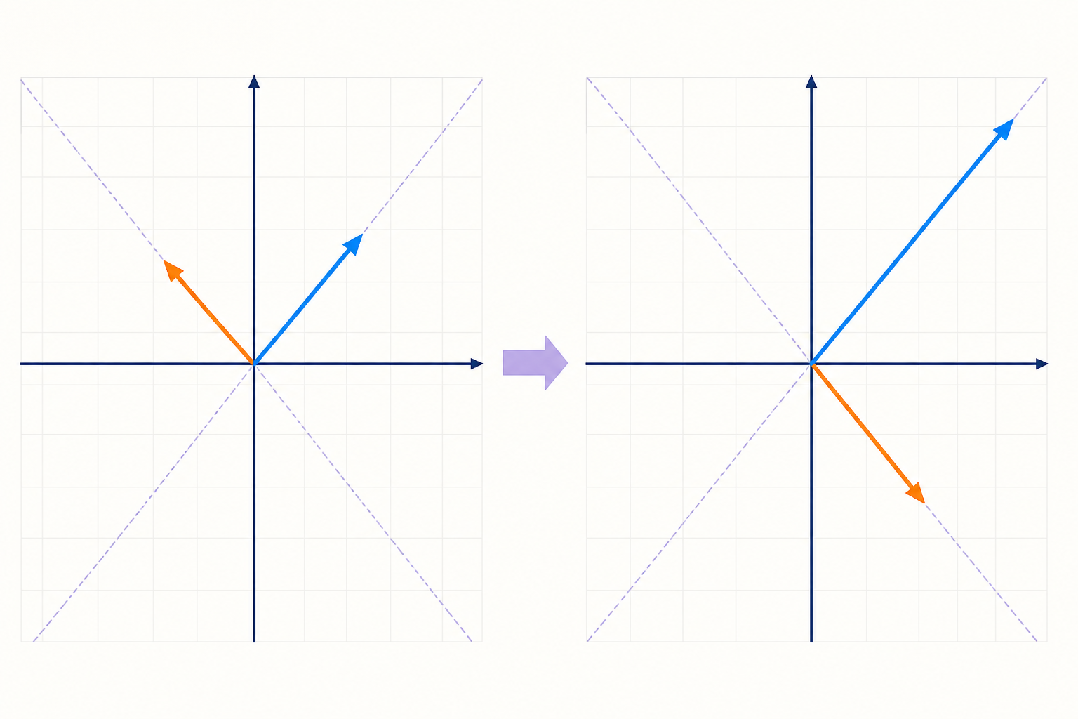Under $A\mathbf v=\lambda\mathbf v$, each eigenvector remains collinear with its original eigendirection. A positive $\lambda$ preserves orientation; a negative $\lambda$ reverses it.

Rearranging the eigenvector equation gives $(A-\lambda I)\mathbf v=\mathbf0$. A non-zero solution exists only when $A-\lambda I$ is singular.

Therefore eigenvalues satisfy the characteristic equation $\det(A-\lambda I)=0$. The determinant produces a polynomial in $\lambda$.

For a $2\times2$ matrix, the characteristic polynomial can be written using trace and determinant: $\lambda^2-\operatorname{tr}(A)\lambda+\det(A)$.

The trace is the sum of diagonal entries. For a $2\times2$ matrix, the eigenvalues sum to the trace and multiply to the determinant, providing a fast check.

To find eigenvalues, form $A-\lambda I$, calculate its determinant, set the result equal to zero and solve the characteristic polynomial.

Exact factorization is preferred when possible. If the polynomial does not factor simply, use the quadratic formula or an approved GDC as appropriate.

A triangular matrix has eigenvalues equal to its diagonal entries, including repetitions. This follows because its determinant is the product of diagonal factors.

A real matrix may have complex eigenvalues. For real diagonalization, enough independent real eigenvectors are required; otherwise work over the complex numbers only if the course context permits it.

For each eigenvalue $\lambda$, solve the homogeneous system $(A-\lambda I)\mathbf v=\mathbf0$. The non-zero solutions form the eigenspace.

Because $\lambda$ is an eigenvalue, $A-\lambda I$ is singular. One equation will be dependent in a typical $2\times2$ case, leaving a free parameter.

Choose a convenient non-zero value for the free parameter to obtain a simple representative eigenvector. Fractions may be cleared by multiplying the whole vector by a common factor.

Verify the result directly with $A\mathbf v=\lambda\mathbf v$.

An eigenvector answer is not unique. If $\mathbf v$ works, every non-zero multiple $c\mathbf v$ works for the same eigenvalue.

The eigenspace includes all these multiples and the zero vector, so it is a subspace even though the zero vector itself is not called an eigenvector.

For an eigenvalue $\lambda$, the geometric multiplicity is the dimension of its eigenspace. This number is at least 1 and no greater than the algebraic multiplicity.

When comparing calculator and written eigenvectors, test whether they are non-zero scalar multiples before deciding they disagree.

Eigenvectors belonging to distinct eigenvalues are linearly independent. Therefore an $n\times n$ matrix with $n$ distinct eigenvalues has enough independent eigenvectors to be diagonalizable.

A repeated eigenvalue may still have enough eigenvectors, but this must be checked. Its geometric multiplicity may equal or be smaller than its algebraic multiplicity.

The matrix $\lambda I$ has the repeated eigenvalue $\lambda$ and every non-zero vector is an eigenvector, so it is diagonalizable.

A Jordan-type matrix such as $\begin{pmatrix}3&1\\0&3\end{pmatrix}$ has only one independent eigenvector and is not diagonalizable.

A square matrix is diagonalizable when it is similar to a diagonal matrix: $A=PDP^{-1}$, where $P$ is invertible and $D$ is diagonal.

The columns of $P$ are linearly independent eigenvectors of $A$. The matching diagonal entries of $D$ are their eigenvalues in the same order.

An $n\times n$ matrix is diagonalizable exactly when it has $n$ linearly independent eigenvectors over the chosen scalar field.

Diagonalization is a change of coordinates to an eigenvector basis. In those coordinates, the matrix acts by independent scalar multiplications.

Start by finding every eigenvalue and a basis for each eigenspace. Confirm that the required number of independent eigenvectors is available.

Form $P$ from the eigenvector columns and $D$ from the matching eigenvalues. Then compute $P^{-1}$.

Verify with $AP=PD$ or reconstruct $PDP^{-1}$. The first check often requires less arithmetic.

A diagonalization is not unique because eigenvectors may be rescaled or reordered, provided $P$ and $D$ remain paired consistently.

If $A=PDP^{-1}$, then repeated factors telescope: $A^n=PD^nP^{-1}$ for non-negative integers $n$.

Powers of a diagonal matrix are easy: raise each diagonal entry to the power while the off-diagonal zeros remain zero.

This method is especially efficient for large powers, symbolic formulas and long-term models. It also reveals which eigenvalue dominates repeated behaviour.

For negative integer powers, $A$ must be invertible, meaning no eigenvalue is zero.

When eigenvectors form a basis, every state vector can be written as a linear combination $\mathbf{x}_0=c_1\mathbf v_1+\cdots+c_n\mathbf v_n$.

The coefficient vector is $\mathbf c=P^{-1}\mathbf{x}_0$. Repeated action then scales each eigencomponent independently.

Thus $A^n\mathbf{x}_0=c_1\lambda_1^n\mathbf v_1+\cdots+c_n\lambda_n^n\mathbf v_n$. This form often explains a model more clearly than a large matrix product.

A component with coefficient zero is absent, so even a dominant eigenvalue has no effect on an initial state lying entirely in other eigenspaces.

A repeated linear transformation follows $\mathbf{x}_{n+1}=A\mathbf{x}_n$, so $\mathbf{x}_n=A^n\mathbf{x}_0$. Diagonalization converts this repeated matrix action into independent scalar powers.

Eigendirections are invariant under every iteration. Their components grow, decay, persist or alternate according to the corresponding eigenvalues.

The eigenvalue with largest absolute value often determines the long-term direction after suitable normalization, provided its eigencomponent is present and uniquely dominant.

This analysis supports iterative graphics, repeated geometric maps, coupled quantities and discrete-time dynamic models.

Eigenvalues classify component behaviour in a discrete model. Values with $|\lambda|<1$ decay, $|\lambda|>1$ grow, $\lambda=1$ persist and $\lambda=-1$ alternate without changing magnitude.

A zero equilibrium of $\mathbf{x}_{n+1}=A\mathbf{x}_n$ is asymptotically stable when every eigenvalue has absolute value less than 1, assuming the matrix can be analyzed in the required setting.

If any present eigencomponent has eigenvalue magnitude greater than 1, that component grows. Model interpretation determines whether this represents population growth, amplification or instability.

Eigenvalue conclusions depend on the model being linear and its parameters remaining constant across iterations.

For a column-state transition model, $\mathbf{x}_{n+1}=T\mathbf{x}_n$. A steady state is an eigenvector for eigenvalue 1 because $T\mathbf{s}=\mathbf{s}$.

When the other eigenvalues have absolute value less than 1, their components decay, leaving the steady-state component in the long term.

For a probability state, normalize the steady-state eigenvector so its entries sum to 1. For a closed population, scale it to the conserved total.

Diagonalization provides an exact formula for the state at step $n$, not just repeated calculator approximations.

Store the square matrix carefully, then use eigenvalue and eigenvector commands if the approved GDC provides them. Menu names and normalization conventions differ by model.

If direct eigen commands are unavailable, calculate $\det(A-\lambda I)$, solve the characteristic polynomial, and use RREF on $A-\lambda I$ for each eigenvalue.

A calculator may return normalized decimal eigenvectors. Compare directions using component ratios and verify with the residual $A\mathbf v-\lambda\mathbf v$.

For diagonalization, construct $P$ and $D$ in matching order, then check $AP=PD$ or $PDP^{-1}=A$.

Use direct $A^n$ as a numerical check, while showing $PD^nP^{-1}$ when diagonalization is the required method.

Common errors include allowing the zero vector, subtracting $\lambda$ from off-diagonal entries, pairing eigenvectors with the wrong eigenvalues and assuming every repeated eigenvalue prevents diagonalization.

A complete solution separates the stages: characteristic equation, eigenvalues, eigenspaces, independence check, construction of $P$ and $D$, then verification.

For powers, write $A^n=PD^nP^{-1}$ and raise only the diagonal entries of $D$. For a state model, interpret the eigencomponents, signs, units and long-term limits.

Use trace and determinant checks for $2\times2$ matrices and use $AP=PD$ to verify eigenpair order efficiently.

Attempt every question before reading the steps. The sequence moves from eigenpair verification to characteristic equations, diagonalization, powers and applied transition models.

Give exact eigenvalues and a convenient exact eigenvector unless approximation is explicitly requested. Verify pairings and interpret model behaviour in context.

Eigenvalues and eigenvectors reveal the directions in which a matrix acts by pure scaling. Diagonalization changes to an eigenvector basis, making powers and repeated models much simpler.

Use the summary as a final checklist: find, pair, verify, diagonalize, apply and interpret.