Solving equations with technology

For one-variable equations, the words root and zero refer to a value $x=r$ for which $h(r)=0$. On the graph $y=h(x)$, the point $(r,0)$ is an $x$-intercept.

Any equation $f(x)=g(x)$ can be rearranged to $h(x)=f(x)-g(x)=0$. Therefore the same solution can be found either where $y=f(x)$ and $y=g(x)$ intersect, or where $y=h(x)$ meets the $x$-axis.

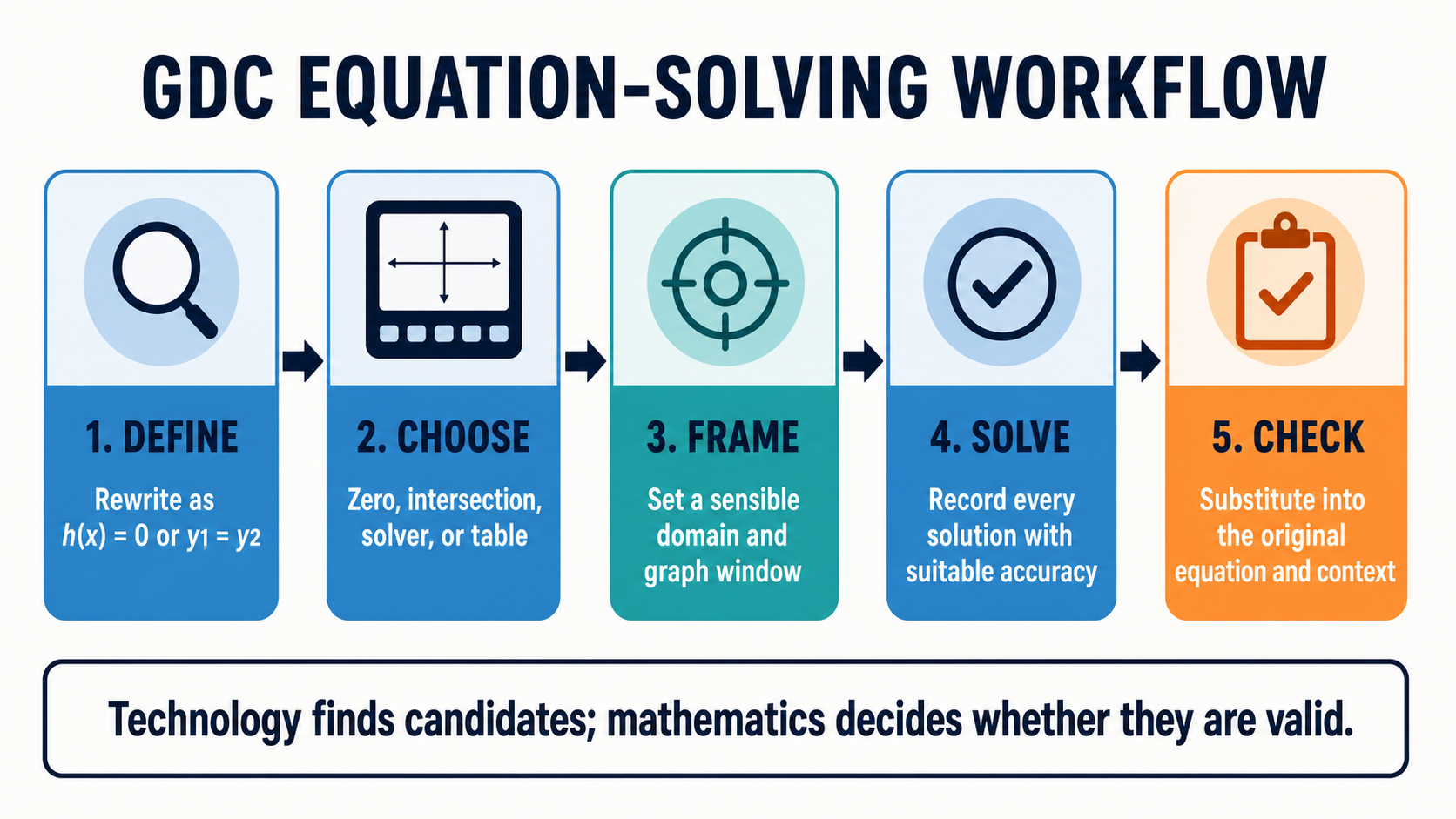Technology finds candidates; mathematical checking determines whether they are valid solutions.

The zero form is often convenient when a GDC has a root or polynomial tool. The intersection form is often more natural when the two sides represent different real-world quantities, such as revenue and cost.

A numerical solver searches for decimal values that make an equation approximately true. Different calculators may use different internal algorithms, but the student workflow is stable: define the equation, restrict the search, choose a method, calculate candidates, and check them.

Start by forming either $h(x)=0$ or $f(x)=g(x)$. Estimate where solutions may lie using algebra, context, a graph or a table. A solver may need an initial guess or lower and upper bounds; poor choices can lead to a different root or no result.

After solving, keep more digits than you plan to report. Substitute the unrounded value into the original equation, then round only the final result according to the question.

A numerical method can miss roots when the search interval is too narrow, when the graph only touches the axis, or when multiple roots lie near one another. A complete solution needs deliberate searching, not one button press.

To solve $h(x)=0$ graphically, enter $Y_1=h(x)$, display a suitable window, and use the GDC zero/root command. The cursor or bracket should enclose the intended root. Record the $x$-coordinate, not merely the screen point.

A graph crossing the axis usually indicates a sign change. A repeated root may only touch the axis and turn around, so a sign-change table can miss it. Zooming near a suspected tangency and using a polynomial solver provide useful confirmation.

A graph is an approximation. Pixel resolution and an unsuitable scale can make close roots appear as one root or a shallow crossing appear to miss the axis. Use a numerical command for the final decimal.

To solve $f(x)=g(x)$, enter $Y_1=f(x)$ and $Y_2=g(x)$, display both graphs, and use an intersection command. The calculator returns a point $(x,y)$; the equation's solution is normally the $x$-coordinate.

Intersection methods are especially useful when each side has a contextual meaning—for example, revenue and cost, supply and demand, or two competing population models. The full point may then be meaningful.

As with roots, there may be several intersections. Pan, zoom, change the domain, and use a table of differences to make sure the full relevant domain has been searched.

A value table is useful when a graph scale hides detail or a numerical solver needs bounds. Evaluate the zero function at regularly spaced inputs and look for values close to zero or a change of sign.

If $h$ is continuous and $h(a)h(b)\lt0$, then at least one root lies between $a$ and $b$. This sign-change test locates a bracket but does not prove there is exactly one root.

Reduce the table step size to narrow the interval. A coarse table can skip two nearby crossings, and it can miss a touching root because no sign change occurs.

For an intersection $f(x)=g(x)$, tabulate both functions or tabulate $h(x)=f(x)-g(x)$. A sign change in $h$ brackets an intersection.

A graph window is not the mathematical domain. It is only the portion of the coordinate plane displayed. If a solution lies outside the window, the graph can falsely appear to have no solution.

Choose the x-range from algebra or context. Time usually begins at zero; a probability lies between zero and one; a count may need to be a non-negative integer. Then estimate a y-range that includes the important outputs of every graphed function.

Use zoom, trace, tables and autoscale as exploration tools, but check their results. Autoscale may create an unhelpful view when one extreme value compresses the rest of the graph.

After finding solutions in one window, expand the domain or justify why no additional solutions are relevant. This is especially important for higher-degree polynomials and periodic functions.

A system of linear equations asks for values that satisfy every equation simultaneously. In two variables, the solution is an ordered pair $(x,y)$; in three variables, it is an ordered triple $(x,y,z)$.

AI HL requires technology for systems in up to three variables. Enter equations in a consistent variable order and standard form. A missing variable has coefficient zero, and constants belong on the correct side.

For a $2\times2$ system, graphing the two lines makes the solution visible as an intersection. For a $3\times3$ system, a simultaneous-equation solver is normally more efficient.

Current AI HL examination systems are designed to have a unique solution, but you must still substitute the ordered values into all original equations.

A polynomial equation can be written as $a_nx^n+a_{n-1}x^{n-1}+\cdots+a_1x+a_0=0$, where $a_n\ne0$. A degree-$n$ polynomial has at most $n$ distinct real roots.

A polynomial solver normally asks for coefficients in descending powers. Enter zero for every missing power. For example, the coefficient list for $2x^4-5x+7=0$ is $2,0,0,-5,7$.

Decide whether the question needs real roots only. Some calculators display complex roots; a graph of a real function shows only real x-intercepts. AI HL problems often require interpreting real solutions in context.

Use a graph to understand the number and location of real roots, then use the polynomial or zero tool for accurate values. Check approximate roots by evaluating the polynomial.

Nonlinear equations include powers, roots, reciprocals, absolute values, exponentials and logarithms. The same graph/solver workflow applies, but restrictions become especially important.

Write restrictions before solving: denominators cannot equal zero; even roots require non-negative radicands; logarithm arguments must be positive. Transformations such as squaring or multiplying by an expression can create extraneous solutions.

A GDC may return a value outside the original domain or may fail near a discontinuity. Always substitute into the original—not merely a rearranged or squared equation.

Exponential and logarithmic equations often have no convenient solution using elementary algebra alone. A graph, intersection command or numerical solver can find the required decimal efficiently.

For exponential models, identify the meaningful domain, often $t\ge0$. For logarithmic equations, enforce positive arguments before interpreting any output.

When an exact logarithmic rearrangement is available, it provides a useful check. Technology should still be used to evaluate the decimal accurately and to investigate more complicated models.

An exact solution represents the value without rounding, such as $x=\sqrt3$ or $x=\frac{7}{4}$. An approximate solution is a rounded decimal, such as $x\approx1.732$.

If a question asks for an exact value and the structure is recognizable, give the exact form. A numerical graph or solver cannot turn a rounded decimal back into a proven exact answer.

If the question requests a decimal or the equation has no elementary exact form, keep guard digits and round the final answer to the required significant figures or decimal places.

Context may determine the final form: money usually uses two decimal places; measurements use appropriate significant figures; counts may require a whole-number threshold rather than ordinary rounding.

A solver message such as “no solution,” “no sign change” or “did not converge” describes the attempted computation, not necessarily the mathematics. Check the window, bounds, initial guess, mode and equation entry before drawing a conclusion.

Validate a numerical root $r$ by computing a residual $R=|h(r)|$, or for $f(x)=g(x)$, $R=|f(r)-g(r)|$. A small residual supports the numerical accuracy but does not replace domain and context checks.

For a linear system, substitute the entire ordered pair or triple into every equation. For a polynomial, confirm all reported real roots and compare the number of roots with the graph and degree.

Interpret the sign and units. A negative time, non-integer item count, probability outside [0,1], or negative length may be mathematically computed but contextually impossible.

Menu names vary between TI-Nspire, TI-84, Casio ClassWiz and Casio graphing models. Learn the equivalent operations on your own approved calculator rather than memorizing one brand's key sequence.

Before any method, clear or inspect stored functions, use parentheses carefully, select real or complex mode as appropriate, and confirm angle mode when trigonometric expressions appear.

For graph zero: enter one zero function, set the window, display the graph, choose Zero/Root and bracket the crossing. For intersection: enter both functions and select the intended crossing. For tables: select a start and step that suit the search.

For polynomial and simultaneous-equation tools: select the correct degree or number of unknowns, enter coefficients in a fixed order, use zero placeholders, solve, and verify in the original equation or system.

Technology questions still assess mathematical communication. Define variables, show the equation or system, state the domain or restrictions, identify the technological method, report all valid solutions, and interpret the result.

Common input mistakes include omitted brackets, missing multiplication signs, incorrect powers, coefficients in the wrong order, failure to enter zero placeholders, and graphing only one side without subtracting the other.

Common search mistakes include using a narrow window, finding only one of several roots, trusting autoscale, using an initial guess near the wrong root, and interpreting “no sign change” as proof of no solution.

Common reporting mistakes include copying the y-coordinate instead of x, rounding too early, using an equals sign for an approximation, retaining an extraneous root, ignoring units, and failing to apply an integer or non-negative constraint.

Attempt each problem with your own GDC before opening the worked method. For technology questions, write enough setup that another student could reproduce the calculation on a different approved calculator.

Unless stated otherwise, give non-exact numerical answers to three significant figures and check them in the original equation.

Define the mathematical equation before opening a calculator. Decide whether a zero, intersection, table, polynomial solver or simultaneous-equation solver is the clearest representation.

Convert $f(x)=g(x)$ into $h(x)=f(x)-g(x)=0$ whenever a zero method is convenient.

For graphs, choose a meaningful domain and window, locate every crossing or tangency, then use a numerical command for accuracy.

For systems and polynomials, preserve variable/power order and enter zero coefficients for missing terms.

Treat outputs as candidates: check the original equation, restrictions, requested accuracy and context before reporting them.